Eigenvectors

Left and right eigenvectors

The word eigenvector formally refers to the right eigenvector x_R. It is defined by the above eigenvalue equation Ax_R = λ_Rx_R, and is the most commonly used eigenvector. However, the left eigenvector x_L exists as well, and is defined by x_LA = λ_Lx_L.

[edit] Characteristic equation

Main article: Characteristic polynomial

When a transformation is represented by a square matrix A, the eigenvalue equation can be expressed as

This can be rearranged to

If there exists an inverse

(A − λI) ^{− 1},

then both sides can be multiplied by the inverse to obtain the trivial solution: x = 0. Thus we require there to be no inverse by assuming from linear algebra that the determinant equals zero:

det(A − λI) = 0.

The determinant requirement is called the characteristic equation (less often, secular equation) of A, and the left-hand side is called the characteristic polynomial. When expanded, this gives a polynomial equation for λ. The eigenvector x or its components are not present in the characteristic equation.

[edit] Example

The matrix

defines a linear transformation of the real plane. The eigenvalues of this transformation are given by the characteristic equation

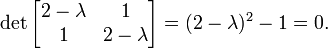
The roots of this equation (i.e. the values of λ for which the equation holds) are λ = 1 and λ = 3. Having found the eigenvalues, it is possible to find the eigenvectors. Considering first the eigenvalue λ = 3, we have

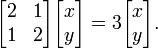
Both rows of this matrix equation reduce to the single linear equation x = y. To find an eigenvector, we are free to choose any value for x, so by picking x=1 and setting y=x, we find the eigenvector to be

We can check this is an eigenvector by checking that :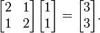 For the eigenvalue λ = 1, a similar process leads to the equation x = − y, and hence the eigenvector is given by

The complexity of the problem for finding roots/eigenvalues of the characteristic polynomial increases rapidly with increasing the degree of the polynomial (the dimension of the vector space). There are exact solutions for dimensions below 5, but for higher dimensions there are generally no exact solutions and one has to resort to numerical methods to find them approximately. For large symmetric sparse matrices, Lanczos algorithm is used to compute eigenvalues and eigenvectors.

[edit] Existence and multiplicity of eigenvalues

For transformations on real vector spaces, the coefficients of the characteristic polynomial are all real. However, the roots are not necessarily real; they may well be complex numbers, or a mixture of real and complex numbers. For example, a matrix representing a planar rotation of 45 degrees will not leave any non-zero vector pointing in the same direction. Over a complex vector space, the fundamental theorem of algebra guarantees that the characteristic polynomial has at least one root, and thus the linear transformation has at least one eigenvalue.

As well as distinct roots, the characteristic equation may also have repeated roots. However, having repeated roots does not imply there are multiple distinct (i.e. linearly independent) eigenvectors with that eigenvalue. The algebraic multiplicity of an eigenvalue is defined as the multiplicity of the corresponding root of the characteristic polynomial. The geometric multiplicity of an eigenvalue is defined as the dimension of the associated eigenspace, i.e. number of linearly independent eigenvectors with that eigenvalue.

Over a complex space, the sum of the algebraic multiplicities will equal the dimension of the vector space, but the sum of the geometric multiplicities may be smaller. In a sense, then it is possible that there may not be sufficient eigenvectors to span the entire space. This is intimately related to the question of whether a given matrix may be diagonalized by a suitable choice of coordinates.

[edit] Shear

Horizontal shear. The shear angle φ is given by k = cot φ.

Shear in the plane is a transformation in which all points along a given line remain fixed while other points are shifted parallel to that line by a distance proportional to their perpendicular distance from the line.^[18] Shearing a plane figure does not change its area. Shear can be horizontal − along the X axis, or vertical − along the Y axis. In horizontal shear (see figure), a point P of the plane moves parallel to the X axis to the place P' so that its coordinate y does not change while the x coordinate increments to become x' = x + k y, where k is called the shear factor.

The matrix of a horizontal shear transformation is . The characteristic equation is λ² − 2 λ + 1 = (1 − λ)² = 0 which has a single, repeated root λ = 1. Therefore, the eigenvalue λ = 1 has algebraic multiplicity 2. The eigenvector(s) are found as solutions of

The last equation is equivalent to y = 0, which is a straight line along the x axis. This line represents the one-dimensional eigenspace. In the case of shear the algebraic multiplicity of the eigenvalue (2) is greater than its geometric multiplicity (1, the dimension of the eigenspace). The eigenvector is a vector along the x axis. The case of vertical shear with transformation matrix is dealt with in a similar way; the eigenvector in vertical shear is along the y axis. Applying repeatedly the shear transformation changes the direction of any vector in the plane closer and closer to the direction of the eigenvector.

[edit] Uniform scaling and reflection

Fig. 3. When a surface is stretching equally in all directions (a homothety) any one of the radial vectors can be the eigenvector.

As a one-dimensional vector space, consider a rubber string tied to unmoving support in one end, such as that on a child's sling. Pulling the string away from the point of attachment stretches it and elongates it by some scaling factor λ which is a real number. Each vector on the string is stretched equally, with the same scaling factor λ, and although elongated, it preserves its original direction. For a two-dimensional vector space, consider a rubber sheet stretched equally in all directions such as a small area of the surface of an inflating balloon (Fig. 3). All vectors originating at the fixed point on the balloon surface (the origin) are stretched equally with the same scaling factor λ. This transformation in two-dimensions is described by the 2×2 square matrix:

Expressed in words, the transformation is equivalent to multiplying the length of any vector by λ while preserving its original direction. Since the vector taken was arbitrary, every non-zero vector in the vector space is an eigenvector. Whether the transformation is stretching (elongation, extension, inflation), or shrinking (compression, deflation) depends on the scaling factor: if λ > 1, it is stretching; if λ <>

[edit] Unequal scaling

1) of a unit square. Eigenvectors are u1 and u2 and eigenvalues are λ1 = k1 and λ2 = k2. This transformation orients all vectors towards the principal eigenvector u1."> 1) of a unit square. Eigenvectors are u1 and u2 and eigenvalues are λ1 = k1 and λ2 = k2. This transformation orients all vectors towards the principal eigenvector u1." src="http://upload.wikimedia.org/wikipedia/commons/thumb/b/be/Unequal_scaling.svg/250px-Unequal_scaling.svg.png" class="thumbimage" border="0" height="188" width="250">

Vertical shrink (k₂ <>k₁ > 1) of a unit square. Eigenvectors are u₁ and u₂ and eigenvalues are λ₁ = k₁ and λ₂ = k₂. This transformation orients all vectors towards the principal eigenvector u₁.

For a slightly more complicated example, consider a sheet that is stretched unequally in two perpendicular directions along the coordinate axes, or, similarly, stretched in one direction, and shrunk in the other direction. In this case, there are two different scaling factors: k₁ for the scaling in direction x, and k₂ for the scaling in direction y. The transformation matrix is , and the characteristic equation is (k₁ − λ)(k₂ − λ) = 0. The eigenvalues, obtained as roots of this equation are λ₁ = k₁, and λ₂ = k₂ which means, as expected, that the two eigenvalues are the scaling factors in the two directions. Plugging k₁ back in the eigenvalue equation gives one of the eigenvectors:

or, more simply, y = 0.

Thus, the eigenspace is the x-axis. Similarly, substituting λ = k₂ shows that the corresponding eigenspace is the y-axis. In this case, both eigenvalues have algebraic and geometric multiplicities equal to 1. If a given eigenvalue is greater than 1, the vectors are stretched in the direction of the corresponding eigenvector; if less than 1, they are shrunken in that direction. Negative eigenvalues correspond to reflections followed by a stretch or shrink. In general, matrices that are diagonalizable over the real numbers represent scalings and reflections: the eigenvalues represent the scaling factors (and appear as the diagonal terms), and the eigenvectors are the directions of the scalings.

The figure shows the case where k₁ > 1 and 1 > k₂ > 0. The rubber sheet is stretched along the x axis and simultaneously shrunk along the y axis. After repeatedly applying this transformation of stretching/shrinking many times, almost any vector on the surface of the rubber sheet will be oriented closer and closer to the direction of the x axis (the direction of stretching). The exceptions are vectors along the y-axis, which will gradually shrink away to nothing.

[edit] Rotation

For more details on this topic, see Rotation matrix.

A rotation in a plane is a transformation that describes motion of a vector, plane, coordinates, etc., around a fixed point. Clearly, for rotations other than through 0° and 180°, every vector in the real plane will have its direction changed, and thus there cannot be any eigenvectors. But this is not necessarily true if we consider the same matrix over a complex vector space.

A counterclockwise rotation in the horizontal plane about the origin at an angle φ is represented by the matrix

The characteristic equation of R is λ² − 2λ cos φ + 1 = 0. This quadratic equation has a discriminant D = 4 (cos² φ − 1) = − 4 sin² φ which is a negative number whenever φ is not equal a multiple of 180°. A rotation of 0°, 360°, … is just the identity transformation, (a uniform scaling by +1) while a rotation of 180°, 540°, …, is a reflection (uniform scaling by -1). Otherwise, as expected, there are no real eigenvalues or eigenvectors for rotation in the plane.

[edit] Rotation matrices on complex vector spaces

The characteristic equation has two complex roots λ₁ and λ₂. If we choose to think of the rotation matrix as a linear operator on the complex two dimensional, we can consider these complex eigenvalues. The roots are complex conjugates of each other: λ_1,2 = cos φ ± i sin φ = e ^{± iφ}, each with an algebraic multiplicity equal to 1, where i is the imaginary unit.

The first eigenvector is found by substituting the first eigenvalue, λ₁, back in the eigenvalue equation:

The last equation is equivalent to the single equation x = iy, and again we are free to set x = 1 to give the eigenvector

Similarly, substituting in the second eigenvalue gives the single equation x = − iy and so the eigenvector is given by

Although not diagonalizable over the reals, the rotation matrix is diagonalizable over the complex numbers, and again the eigenvalues appear on the diagonal. Thus rotation matrices acting on complex spaces can be thought of as scaling matrices, with complex scaling factors.